Estimating Total County Employment for the Humboldt Economic Index:
Two Models by John Manning December 2, 2002 Revised March 31, 2003
Executive Summary
Employment is, arguably, the single most important indicator of economic activity. Thus, a timely and accurate estimation of the employment level is of value for planning and decision-making. Presently, the California Employment Development Department estimates total employment in each of the state's 58 counties every month. The EDD's preliminary estimates for a given month are usually posted within two weeks of that month's end and the final estimates are available some four weeks later. As a result, anyone interested in local employment trends must deal with a two to six week lag.
The two models presented here attempt to provide an accurate estimate of total Humboldt County employment for the current month, two to three weeks before the preliminary EDD figure is available. The first uses a variety of lagged employment, lagged retail, lagged lumber-based manufacturing, and lagged help-wanted advertising data compiled for the Humboldt Economic Index as the independent variables in its regression equation. The second is based on lagged employment, lagged help-wanted advertising and lagged claims for unemployment insurance.
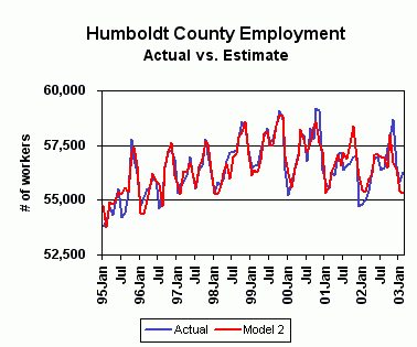
The relative strength of Model 2 is apparent when the two models' performance is compared. Model 2's estimation of monthly employment (the number of people employed in a given month) is significantly more accurate than Model 1's. There is an 88.4 percent correlation between actual employment and Model 2's estimate for the period January 1995 to February 2003, and The average deviation between it's estimate and the actual employment level over this same period is 21 percent smaller than the same deviation arising from Model 1. This means the information provided by the retail and manufacturing data in the first model is less valuable then that provided by the unemployment insurance claims data in the second. However, given the sometimes high deviation of Model 2's estimate, it cannot always be relied upon to provide useful information. A more general sense of labor market activity can be gleaned by looking at just the direction of month-over-month movement. Over the same period, Model 2 correctly predicted whether there would be a net increase or decrease in total county employment 83.9 percent of the time, compared to Model 1's 73.1 percent accuracy. While Model 2 appears to be slightly more accurate, there is no statistically significant difference between the two models in this case.
Nevertheless, Model 2 is the stronger model overall and it alone will be presented as part of the monthly report of the Humboldt Economic Index along with current information regarding its accuracy so that readers can judge for themselves the value of its prediction.
No econometric model can accurately predict unanticipated economic shocks. Unforeseen disruptions can negatively impact a model's ability to provide quality information. This can be observed in how the two models handled the shock of September 11, 2001. In the event of further shocks, the effectiveness of the model should be reassessed.
Introduction
The Humboldt Economic Index is a monthly barometric indicators project that has tracked the local economy since January 1994. Data are collected each month from about two dozen distinct sources categorized within six sectors. These data are then used to compute a composite index showing the current level of local economic activity relative to any month during the past eight years. The Index's six sectors are electricity consumption, total county employment, home sales, hospitality, lumber-based manufacturing, and retail.
Since the local employment sector carries a comparatively greater weight than the other five sectors in computing the composite index, it is, arguably, the most important single indicator of economic activity. Thus, it would be valuable to have an accurate estimation of current countywide employment as soon as possible in order to get a sense of where the local economy is headed.
Presently, the California Employment Development Department estimates total employment in each of the state's 58 counties every month. The EDD's preliminary estimates for a given month are usually posted within two weeks of that month's end and the final estimates are available some four weeks later. As a result, anyone interested in local employment trends must deal with a two to six week lag.
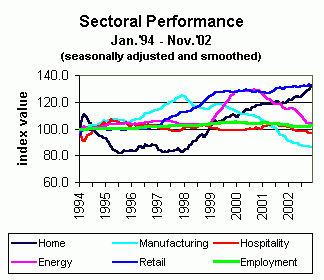
This relative stability, and the need for a timelier estimate, makes the local employment sector an ideal subject for regression analysis.Over the life of the Index, employment has been, by far, its most stable sector:
The two models presented here attempt to provide an accurate estimate of total Humboldt County employment for the current month, two to three weeks before the preliminary EDD figure is available.
The Models
Both models are relatively simple regression-based estimators of total county employment in the current month. Model 1 uses a variety of lagged employment, lagged retail, lagged lumber-based manufacturing, and lagged help-wanted advertising data compiled for the Humboldt Economic Index as the independent variables in its regression equation. Because timely data are not always available in the current month for the retail and lumber-based manufacturing sectors, and because over time some participating firms may go out of business or chose to end their association with the project, a second model was developed using data from sources whose long-term reliability is more likely. Model 2 is based on lagged employment, lagged help-wanted advertising and lagged claims for unemployment insurance. Both models were generated using data from January 1994 to June 2002.
Model 1:
Estimated Employment(t) = 33431 + 0.411 E(t-1) - 0.155 E(t-9) - 21.7 R(t-4) + 39.4 R(t-6) + 18.8 R(t-11) + 21.2 M(t-2)
- + 13.0 HWA(t-1) + 13.3 HWA(t-2) + 9.34 HWA(t-7) - 24.3 HWA(t-8)
where:
- t represents the current month
- E(t-i) represents the number of people employed in Humboldt County i months ago as determined by the EDD.
- R(t-i) represents the not seasonally adjusted index value for the retail sector i months ago as determined the Humboldt Economic Index.
- M(t-i) represents the not seasonally adjusted index value for the lumber-based manufacturing sector i months ago. Because this value is not directly computed as part of the Humboldt Economic Index, it is computed here using the monthly not seasonally adjusted index values for board footage of lumber shipped and lumber-based manufacturing payroll. (NSA lumber-based manufacturing index value = (0.7 * NSA board foot index value) + (0.3 * NSA payroll index value)).
- HWA(t-i) represents the mean of the raw counts of help-wanted advertisements appearing in the Eureka Times-Standard i months ago on the second and fourth Sundays of that month.
Example: if t = January 1995, then t-1 = December 1994, t-2 = November 1994, ... , t-12 = January 1994.
Initial data used to run the regression were from the time period January 1994 through June 2002:
- E(t-1, t-2, ... , t-12)
- R(t-1, t-2, ... , t-12)
- M(t-1, t-2, ... , t-12)
- HWA(t-1, t-2, ... , t-12)
Model 1 Variables | |||
Variable | Range | t-value* | |
--- | Minimum Value | Maximum Value | --- |
| Constant** | 53,800 | 59,200 | 7.29 |
| E(t-1) | 53,800 | 59,200 | 6.53 |
| E(t-9) | 53,800 | 59,200 | -2.33 |
| R(t-4) | 95.2 | 165.8 | -3.96 |
| R(t-6) | 95.2 | 165.8 | 6.40 |
| R(t-11) | 90.2 | 165.8 | 3.13 |
| M(t-2) | 75.1 | 152.6 | 4.68 |
| HWA(t-1) | 65.0 | 158.0 | 3.12 |
| HWA(t-2) | 65.0 | 158.0 | 3.36 |
| HWA(t-7) | 65.0 | 158.0 | 2.41 |
| HWA(t-8) | 65.0 | 158.0 | -5.84 |
| * Significance occurs at t(0.05, 74) = +1.6657 or -1.6657. | |||
| ** Constant refers to the dependent variable,Employment(t). |
Other statistical information:
- Number of observations (n): 86
- F-value: 45.84
- r-squared: 85.9%
- Adjusted r-squared: 84.1%
- Durbin-Watson: 1.90
- Random residuals: Yes
- Normally distributed residuals: Yes
There was no apparent multicollinearity between the independent variables, which suggests that each is contributing more or less unique information to the model.
The model began with 89 observations and 48 independent variables. There were a few outlying observations in some of the manufacturing variables, but there was no compelling reason to omit them. None of them had an unusually high impact when the regressions were run. Furthermore, this sector of the economy has traditionally been one of boom or bust and is currently experiencing serious structural decline, so it makes a certain amount of sense to leave the extremes in the model. The one surviving manufacturing variable has one outlying observation on the low end of its range. Three observations were omitted due to their unusually high residuals. All of the omitted independent variables were removed due to their insignificant t-values.
The F-value of 45.84 is fairly strong, and it indicates that the model's independent variables, taken together, are significantly predictive of current employment. Additionally, the adjusted r-squared of 84.1 indicates that this package of independent variables accounts for well over four-fifths of the variability of the dependent variable. Overall, this is a strong model.
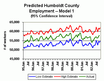
95% Confidence Interval:
The extremes of this interval were determined by applying the following expressions to the constant and each of the independent variables:
Lower extreme of the interval:
- Coefficient - (t(0.025 , n - 2))(std. dev. / sqrt(n))
Estimated Employment(t) = 32447 + 0.398 E(t-1) - 0.169 E(t-9) - 22.8 R(t-4) + 38.1 R(t-6) + 17.5 R(t-11)
- + 20.2 M(t-2) + 12.1 HWA(t-1) + 12.5 HWA(t-2) + 8.5 HWA(t-7) - 25.2 HWA(t-8)
Upper extreme of the interval:
- Coefficient + (t(0.025 , n - 2))(std. dev. / sqrt(n))
Estimated Employment(t) = 34415 + 0.425 E(t-1) - 0.141 E(t-9) - 20.5 R(t-4) + 40.7 R(t-6) + 20.1 R(t-11)
- + 22.1 M(t-2) + 13.9 HWA(t-1) + 14.2 HWA(t-2) + 10.2 HWA(t-7) - 23.4 HWA(t-8)
Actual refers to actual total Humboldt County employment
Model 2:
Estimated Employment(t) = 14767 + 0.494 E(t-1) + 0.349 E(t-11) - 7.28 HWA(t-3) - 17.2 HWA(t-8) - 1.06 UIC(t-1) - 0.482 UIC(t-2) - 1.18 UIC(t-8) + 0.554 UIC(t-11)
where:
- t represents the current month
- E(t-i) represents the number of people employed in Humboldt County i months ago as determined by the EDD.
- HWA(t-i) represents the mean of the raw counts of help-wanted advertisements appearing in the Eureka Times-Standard i months ago on the second and fourth Sundays of that month
- UIC(t-i) represents the monthly raw counts of new claims for unemployment insurance i months ago as provided by the Employment Development Department.
Initial data used to run the regression were from the time period January 1994 through June 2002:
- E(t-1, t-2, ... , t-12)
- HWA(t-1, t-2, ... , t-12)
- UIC(t-1, t-2 , ... , t-12)
| Model 2 Variables | |||
|---|---|---|---|
| Variable | Range | t-value* | |
| --- | Minimum Value | Maximum Value | --- |
| Constant** | 53,800 | 59,200 | 3.18 |
| E(t-1) | 53,800 | 59,200 | 8.42 |
| E(t-11) | 53,400 | 59,200 | 5.47 |
| HWA(t-3) | 65.0 | 158.0 | -1.80 |
| HWA(t-8) | 81.0 | 158.0 | -4.53 |
| UIC(t-1) | 722 | 2185 | -4.09 |
| UIC(t-2) | 722 | 2185 | -1.94 |
| UIC(t-8) | 722 | 2185 | -5.42 |
| UIC(t-11) | 722 | 2185 | 3.23 |
| * Significance occurs at t(0.05, 76) = +1.6652 or -1.6652. | |||
| ** Constant refers to the dependent variable,Employment(t). |
Other statistical information:
- Number of observations (n): 85
- F-value: 56.11
- r-squared: 85.5
- Adjusted r-squared: 84.0
- Durbin-Watson: 2.28
- Random residuals: Yes
- Normally distributed residuals: Yes
There was no apparent multicollinearity between the independent variables, which suggests that each is contributing more or less unique information to the model.
The model began with 89 observations and 36 independent variables There were no outlying observations. Four observations were omitted due to their unusually high residuals. All of the omitted independent variables were removed due to their insignificant t-values.
The F-value of 56.11 is slightly stronger than in model 1, and it indicates that this model's independent variables, taken together, are significantly predictive of current employment. Although this model's adjusted r-squared, at 84.0, is slightly weaker than that of model 1, it too indicates that this package of independent variables accounts for well over four-fifths of the variability of the dependent variable. Thus, this also is a strong model.
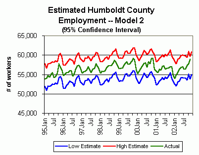
95% Confidence Interval:
The extremes of this interval were determined by applying the following expressions to the constant and each of the independent variables:
Lower extreme of the interval:
- Coefficient - (t(0.025 , n - 2))(std. dev. / sqrt(n))
Estimated Employment(t) = 13765 + 0.482 E(t-1) + 0.335 E(t-11) - 8.16 HWA(t-3) - 18.1 HWA(t-8)
- - 1.12 UIC(t-1) - 0.536 UIC(t-2) - 1.22 UIC(t-8) + 0.517 UIC(t-11)
Upper extreme of the interval:
- Coefficient + (t(0.025 , n - 2))(std. dev. / sqrt(n))
Estimated Employment(t) =15769 + 0.507 E(t-1) + 0.362 E(t-11) - 6.41 HWA(t-3) - 16.4 HWA(t-8) - 1.01 UIC(t-1) - 0.428 UIC(t-2) - 1.13 UIC(t-8) + 0.591 UIC(t-11)
Analysis
Actual refers to actual total Humboldt County employment
In February 2003, the EDD revised the manner in which it tallies total county employment. Consequently, the Humboldt Economic Index updated its employment sector data series using revised data. While the following analysis is based on these new numbers, the models themselves are still based on the old data since the regressions were run prior to the revision. Obviously, this fact introduces a disconnect of sorts because the coefficient of each term in the two models was derived from a slightly different data series than the series currently used as part of the models' input. It is not known precisely how much of an effect this has on the accuracy of the estimates, though it is assumed that accuracy is reduced at least minimally. However, since the results remain favorable (see the analysis below), the regressions will not be re-run for the time being.
The two models were tested against actual total Humboldt County employment using data from January 1995 through February 2003. The results are explained below.
Model 1:
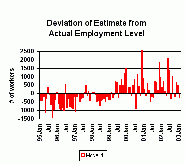
When compared to the EDD's employment numbers, model 1 correlated to actual performance at the 86.4 percent level. The deviation of this model's estimate from the actual level each month ranged from -1,439 to 2,699, with an average deviation (absolute value) of 531.
Model 2:
This model performed noticeably better when its estimations were compared to the EDD's figures over the same period. Model 2 correlated to actual employment data at the 88.4 percent level. The range of the deviation of its estimate from the actual level each month was tighter than the first model's -- -1,951 to 1,1426 -- and its average deviation each month was 21 percent smaller at 419.
Model 2's apparent superiority was tested to determine whether the two models' abilities to estimate the employment level are different at a statistically significant level. Since the two samples are dependent, a two tail, paired t-test was run on the absolute values of the differences between each model's estimate and the actual level of employment for each month using data from January 1995 through June 2002. The critical value for this test is t(0.025 , 97) = -1.9847 or +1.9847. With a t-value of -2.04, the test shows there is a statistically significant difference between the models at the 0.05 level.
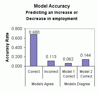
Model 2 comparative strength is evident again when the two models are used to predict whether the current month's employment level will be an increase or decrease from the previous month's level. Using data from January 1995 through February 2003, model 1 correctly predicted an increase or decrease 74.2 percent of the time. Model 2 was accurate 82.4 percent of the time. Over this period, the two models agreed in their predictions 79.3 percent of the time (0.680 + 0.113). When this occurred, the prediction was correct 86.8 percent of the time (0.680 / 0.793). The models disagreed 20.6 percent of the time (the agreement and disagreement don't add up to 1.000 due to rounding). In these cases, model 2 was more than twice as accurate as model 1 -- 14.4 percent versus 6.2 percent. These results are summarized in the chart below:
To determine whether Model 2 is significantly better at predicting changes in the direction of employment growth, a two tail Wilcoxon test was run on the models' respective accuracy. The test was run using each model's performance in predicting up or down movement in the level of employment from one month to the next. A correct prediction was assigned a value of 1 and an incorrect prediction was assigned a value of 0. Data used were from January 1995 through February 2003. Here, the critical value, at the 0.05 level, is p = 0.05. The test resulted in p = 0.121. Therefore, there is no statistically significant difference between the two models' abilities to predict the direction of month-over-month movement.

Other Models
A number of other models using various data available to the Humboldt Economic Index were tried unsuccessfully (for one reason or another, they were not significant estimators of the dependent variable). These included:
- using the same initial set of variables as in model 1 with the addtion of UIC(t-1, t-2, ... , t-12).
- using the Index's leading indicators, individually and in combinations, to predict next month movement in the composite index.
- using the Index's leading indicators, individually and in combinations, to predict next month movement in employment.
Other statistically significant models for estimating employment were developed, but not adopted because their results were substantially weaker than those for the two models presented. These included:
- using a variety of lagged employment data as independent variables.
- using a variety of lagged employment, lagged retail and lagged lumber-based manufacturing data as independent variables.
Issues of Concern
As noted above, the revision of the EDD data series occurred after the regressions the two two models are based on were run. This introduces an unknown level of inaccuracy into the models. At this point, it is assumed that the impact is minimal. Since the measurements of each model's respective accuracy vary slightly from month to month, these results will continue to be monitored in order to determine if modification is necessary.
Furthermore, no econometric model can foresee economic shocks. This can be seen in how these two models handled the shock of September 11, 2001. Both understated the steepness of the decline that followed, and Model 1 overstated the subsequent recovery. Should additional shocks occur, it might be worthwhile to rework the regressions in order to take any significant disruptions into account.
Conclusion
While both models are reasonably good predictors of month-over-month changes in the level of total Humboldt County employment, Model 2 is significantly more accurate over the period January 1995 through February 2003. Unfortunately, given the occasionally high deviation of the Model 2's estimate from the actual level of employment, it cannot always be relied upon to be provide useful information. However, the model's ability to correctly predict changes in the direction of employment growth more than four out of five times can be useful. Consequently, it will be presented as part of the monthly report of the Humboldt Economic Index, along with information on its accuracy so that readers can judge for themselves the value of the estimations and predictions.
Given the concerns noted above, the model's performance will be monitored. If its accuracy eventually falls to the point where the information produced is no longer useful, new regressions can be run.
